Author: Wei Yuanpei
Background
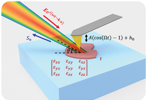
Optical imaging at the nanoscale is one of the cornerstones of nano-optics research. Traditional optical imaging techniques, limited by Abbe's diffraction law, can only achieve a resolution of about half a wavelength, far from meeting the needs of nano-optics research. Scattering-type scanning near-field optical microscopy (s-SNOM) is an effective method for breaking through the optical diffraction limit. By combining near-field optical imaging technology with scanning probe microscopy, the imaging resolution no longer depends on the working wavelength, but on the tip radius (on the order of tens to a hundred nanometers). In s-SNOM imaging, a key issue is the analysis of measurement data. Due to its special working mechanism, the data measured by s-SNOM are difficult to directly relate to the optical and geometric properties of the measured object. To connect the acquired near-field signals with material parameters, a model capable of correlating the two needs to be established. Since s-SNOM was proposed, a variety of analytical models have been developed. This article briefly introduces the models commonly used in s-SNOM analysis.
s-SNOM analytical models
Model 1: PDM
The point dipole model (PDM) is the earliest near-field analytical model proposed [1]. In this model, the probe is approximated as a dielectric sphere, and the interaction of the probe with the sample is described through induced image charges. This model can describe the near-field interaction process reasonably well qualitatively, but its simple approximation leads to shortcomings in quantitative description, and it can only serve as an aid for understanding near-field signals. In this model, the response of the probe is characterized by an effective polarizability:
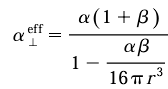
where the terms are the polarizabilities of the probe and the sample, respectively, and r is the distance from the center of the equivalent sphere to the sample half-plane.
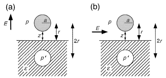
Fig. 1 Probe equivalence in the PDM [1]
On the basis of the PDM, Moon et al. proposed the line dipole model (LDM) [2]. The main improvement of this method over the PDM lies in describing the back-and-forth excitation process between the probe and the sample after the probe excites the sample; this process is described by a series of dipoles at the positions of the probe and the sample. Thus, the dipole moment of the system is:

which includes the dipole moments in the probe (subscript p) and the sample (subscript s); h is the distance from the center of the equivalent sphere to the sample plane, and a is the radius of the equivalent sphere. Since this model accounts for multiple interactions, it is significantly improved over the PDM in quantitative description and can achieve good fitting of experimentally measured near-field data.
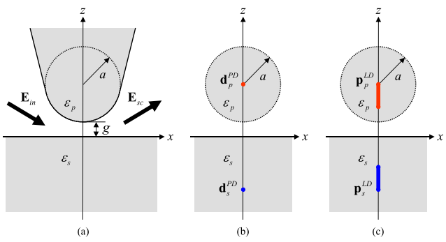
Fig. 2 Probe equivalence in the LDM
To address the problem that the probe parameters in the model need to be determined during the fitting process, Moon et al. also proposed a reference-free calibration method [3]. Since the near-field energy excited under different tip radii of curvature is concentrated in different wavevector ranges and decays at different rates with propagation distance, Moon et al. measured the approach curves of probes with different tip radii (the radii measured by electron microscopy), making it possible to directly obtain the tip radius of the probe in use by measuring the approach curve in experiments.
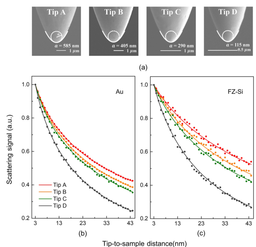
Fig. 3 Different tip radii correspond to different approach curves
Model 2: FDM
The finite dipole model (FDM) is an approximate model proposed by Cvitkovic et al. [4]. Unlike the PDM, the near-field probe in this model is no longer equivalent to a sphere located at the tip, but to an ellipsoid. This model is also based on the image-charge equivalence principle, but takes into account the influence of the probe length, making it more accurate than the PDM. The effective polarizability of the probe in this model is given by:

The formula contains geometric parameters such as the equivalent length of the probe (L), the probe-sample distance (H), and the tip radius of curvature (R), with g being a fitting parameter. In the terahertz band, this model is a commonly used analytical model.
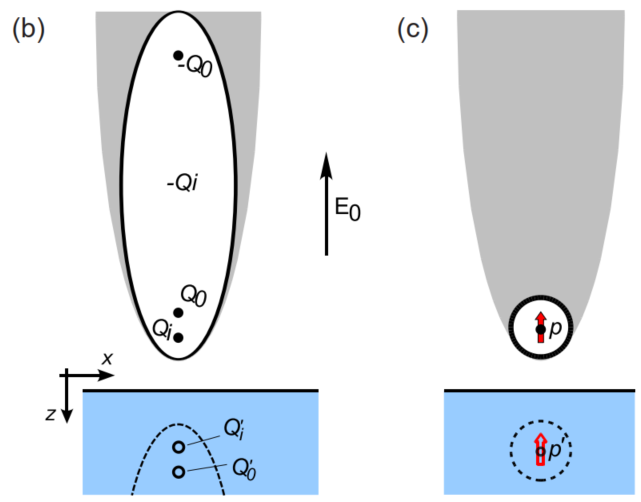
Fig. 4 Probe equivalence in the FDM
Model 3: LRM
Unlike the aforementioned models based on the electrostatic approximation, the lightning rod model (LRM) is another analytical model proposed by McLeod et al. [5]. By considering the actual geometric shape of the probe and using electrodynamic methods, the charge distribution on the probe and the induced polarizability under excitation by the incident field are calculated. The charge distribution on the probe in this model is given by:

In the above equation, the left side is the charge distribution on the probe; the first term on the right is the induced charge distribution generated by a unit incident field, and the second term is the sum of charges induced by near-field components with different momenta. Within it, from left to right, the first term is the charge distribution induced by a unit near field of different momenta, the second term is the weight of near fields of different momenta in the total near field, the numerator of the fraction is obtained by spectral decomposition of the first term, and I is the identity matrix. Since both field retardation and probe shape are taken into account, this model can fit actually measured signals reasonably well. Several extended models have been developed based on this model [6, 7], but because the geometric shape of the probe must be considered, the complex geometry of actual tips is difficult to describe precisely, which affects the analytical effectiveness of this model.
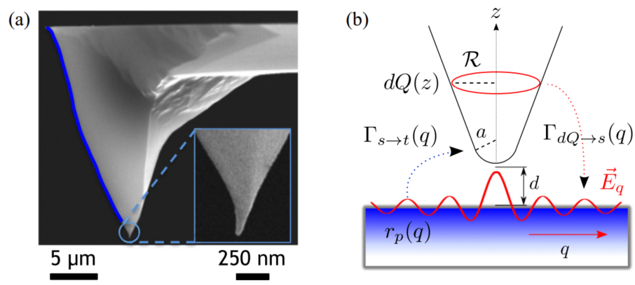
Fig. 5 The LRM analyzes the near-field interaction process based on the actual probe shape
Applications of s-SNOM analytical models
In the analysis of near-field data, applying the aforementioned analytical models allows various pieces of information to be extracted from near-field measurement data, such as the permittivity and thickness of materials [8, 9]. This is because when we demodulate at the tapping frequency of the probe, the near-field signals of different orders contain material properties at different depths — the higher the order, the smaller the probing depth.
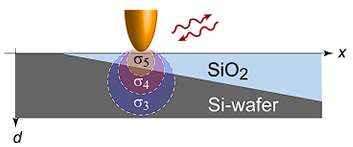
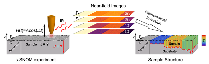
Fig. 6 Extracting optical constants and thickness of materials based on differences between orders
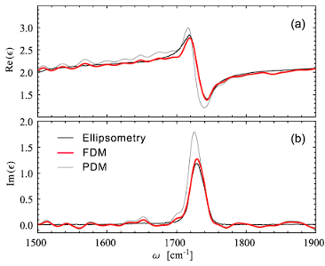
Fig. 7 Broadband extraction of the dielectric function based on an analytical model
Similarly, the dielectric function of materials can also be extracted through inversion methods over a broad spectral range [10]. All these applications rely on establishing an analytical model to analyze the test data.
Summary
Scattering-type scanning near-field optical microscopy (s-SNOM), with its ultra-broadband optical nano-imaging capability from terahertz to visible light and its high-resolution imaging ability, has revealed many novel physical phenomena that cannot be measured by traditional optical and electronic imaging. To fully exploit its capability for nanoscale material characterization, more accurate models describing its working process are still needed to correlate material properties with experimental data. Current methods based on approximate models require parameter fitting, which limits their application. Another possible approach is to incorporate machine learning (ML) [11], but this requires large amounts of data, which also limits its application. If better data analysis methods can be discovered, s-SNOM will surely play an even greater role in future exploration of the nanoworld.
References
[1]Knoll B, Keilmann F. Enhanced dielectric contrast in scattering-type scanning near-field optical microscopy [J]. Optics Communications, 2000, 182(4-6): 321-8.
[2]Moon K, Jung E, Lim M, et al. Quantitative analysis and measurements of near-field interactions in terahertz microscopes [J]. Opt Express, 2011, 19(12): 11539-44.
[3]Moon Y, Lee H, Lim J, et al. Reference-free self-calibrating tip-based scattering-type THz near-field microscopy [J]. AIP Advances, 2023, 13(6).
[4]Cvitkovic A, Ocelic N, Hillenbrand R. Analytical model for quantitative prediction of material contrasts in scattering-type near-field optical microscopy [J]. Opt Express, 2007, 15(14): 8550-65.
[5]McLeod A S, Kelly P, Goldflam M D, et al. Model for quantitative tip-enhanced spectroscopy and the extraction of nanoscale-resolved optical constants [J]. Physical Review B, 2014, 90(8).
[6]Chui S T, Chen X, Liu M, et al. Scattering of electromagnetic waves from a cone with conformal mapping: Application to scanning near-field optical microscope [J]. Physical Review B, 2018, 97(8).
[7]Jiang B Y, Zhang L M, Castro Neto A H, et al. Generalized spectral method for near-field optical microscopy [J]. Journal of Applied Physics, 2016, 119(5).
[8]Govyadinov A A, Mastel S, Golmar F, et al. Recovery of Permittivity and Depth from Near-Field Data as a Step toward Infrared Nanotomography [J]. ACS NANO, 2014, 8(7): 6911-21.
[9]Mooshammer F, Sandner F, Huber M A, et al. Nanoscale Near-Field Tomography of Surface States on (Bi0.5Sb0.5)2Te3 [J]. Nano Letters, 2018, 18(12): 7515-23.
[10]Govyadinov A A, Amenabar I, Huth F, et al. Quantitative Measurement of Local Infrared Absorption and Dielectric Function with Tip-Enhanced Near-Field Microscopy [J]. JOURNAL OF PHYSICAL CHEMISTRY LETTERS, 2013, 4(9): 1526-31.
[11]Chen X, Xu S, Shabani S, et al. Machine Learning for Optical Scanning Probe Nanoscopy [J]. Advanced Materials, 2023, 35(34): 2109171.