Author: Zhang Zhuocheng
Readers of our previous articles already know that scattering-type scanning near-field optical microscopy (s-SNOM) is a microscopy technique that can focus electromagnetic waves — from visible light to terahertz — down to the nanoscale and directly read the "nano-spectral fingerprint" of a sample [1]. The trick is this: the probe taps lightly on the sample surface, and the near-field signal, which is extremely sensitive to the tip–sample distance, is modulated onto the harmonics (nΩ) of the probe vibration. By "unlocking" the signal at these higher harmonics, we can far exceed the diffraction limit and obtain nanoscale imaging and spectroscopy, truly seeing the microscopic structure and composition of the sample.

Today let's talk about a powerful advanced technique: near-field tomography.
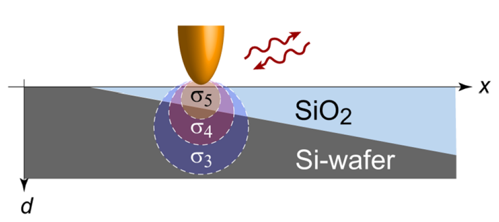
s-SNOM has a very interesting property: each order of the signal we read out (s₁, s₂, s₃...) actually acts like a "perspective filter with a different depth", with different sensitivity to different "depths" of the sample. For example, higher-order signals (such as s₄, s₅) are most sensitive to the sample surface, seeing the composition and structure closest to the surface layer; lower-order signals (such as s₁, s₂) penetrate deeper, carrying signals from buried layers and covering layers. This is the physical basis of near-field tomography: the higher the order, the more surface-sensitive; the lower the order, the deeper the probing.
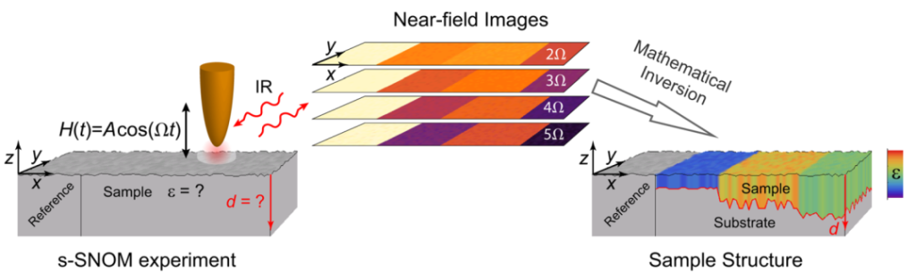
Using this property, we can not only see the surface of a sample, but also "layer by layer" see covering layers and buried layers — almost like a CT scan — reading the sample's "nano-spectral fingerprint" depth by depth. In short, near-field tomography "peels away" surface and buried information layer by layer, truly achieving nanoscale "perspective" and depth discrimination.
Why is it that "the higher the order, the more surface-sensitive"?
There is actually a very interesting physical mechanism behind this. The near-field signal of s-SNOM can be understood as a mixture of evanescent waves with different lateral momenta (q). The larger the momentum q, the faster the field decays and the shallower it penetrates, so it is particularly sensitive only to the vicinity of the surface; the smaller the q, the deeper it can penetrate, probing information inside the sample.
Higher-order near-field signals are essentially more weighted toward these "large-q" components, effectively raising the "signal weight" of the surface; lower-order signals retain more small-q components, and thus can see the composition and structure of deeper layers. This is like using a set of "physical filters" that can distinguish materials layer by layer, from the surface down to the interior.
Correspondingly, high-q near-field waves not only "hug the surface", their electric fields are also more strongly localized, which greatly improves resolution. So higher-order signals are not only more surface-sensitive, but also deliver higher resolution — this is the secret behind near-field microscopy achieving nanoscale, or even sub-20-nanometer, super-resolution.
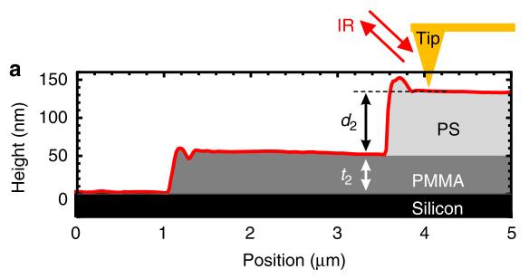
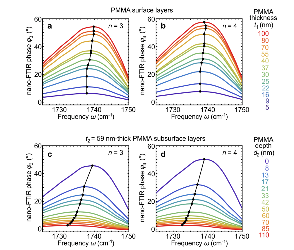
In near-field tomography, we can not only distinguish the signal strength of different layers, but more importantly, we can see that the nano-spectra (e.g., peak positions, line shapes) at different depths change systematically. This is because the spectral peak positions of the near-field signal are governed by the momentum-dependent reflection coefficient β(ω,q). For multilayer structures, β(ω,q) changes with q (i.e., with "depth"), causing resonance peaks to shift systematically with layer position and thickness.
Finally, regarding the calculation method for near-field signals of multilayer samples, the commonly used model is the finite dipole model (FDM), which computes the near-field scattering coefficient. The specific formulas are as follows [3]:
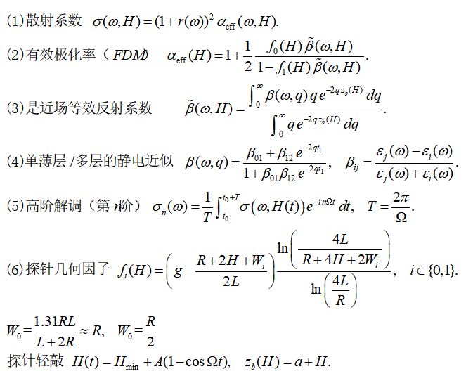
Here, R, L, g: R is the tip radius of curvature, L is the effective length (semi-major axis of the ellipsoid), and g is a dimensionless calibration factor (≈0.6–0.7); a is the effective source height (distance from the effective charge to the surface), taken as a = 1.4R; t₁ is the thickness of the covering layer; εᵢ(ω) is the complex permittivity of each layer (used in the βᵢⱼ calculation); r(ω) is the far-field reflection coefficient of the surface.
References
[1] Hillenbrand, Rainer, et al. "Visible-to-THz near-field nanoscopy." Nature Reviews Materials 10.4 (2025): 285-310.
[2] Govyadinov, Alexander A., et al. "Recovery of permittivity and depth from near-field data as a step toward infrared nanotomography." Acs Nano 8.7 (2014): 6911-6921.
[3] Mester, Lars, et al. "Subsurface chemical nanoidentification by nano-FTIR spectroscopy." Nature communications 11.1 (2020): 3359.